Analyze in the browser

The left drawer of an opened section lists the analyses. Each one runs in your browser, on the data in view, and nothing is sent anywhere to compute it. What it makes is kept with the data: in the unsaved changes until you save a version, then in the version.

The analyses

• Label cells: draw around cells and name them, into a new column (labels unless you name another) or one you have. With the lasso, drag around the cells (each loop adds to the selection when you let go) or click point by point; or drag a circle, ellipse, square or rectangle. While you draw, hold Space and drag to pan.
• Find clusters: Leiden clustering the way scanpy does it by default. Counts are normalized and log-transformed, the most variable genes go into a PCA, and Leiden works on the cells' nearest-neighbor graph. Resolution is yours to set. The report shows each cluster's size and where it is, and how much of the variation the PCA's components hold.
• Compare groups: a Wilcoxon test of every gene between two groups. A group can be a category of any column or the cells you selected on the tissue. A column with more than 100 groups, such as one of cell IDs, can't be compared. The report shows the volcano beside maps of where the two groups are, and each side's strongest genes.
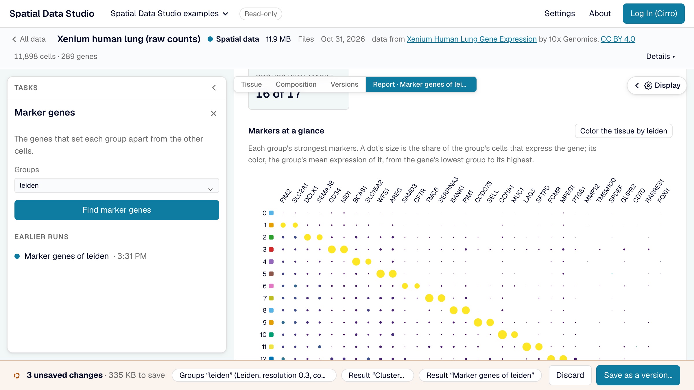
• Marker genes: each group of a column against all the others. The report shows every group's strongest markers in one dot plot, then a card per group: its size, where its cells are, and what marks it.
• Spatially variable genes: Moran's I of every gene over each cell's six nearest neighbors on the tissue. The report maps the strongest genes, and sorts the strongest 60 into spatial patterns: genes whose maps look alike.
• Neighborhood enrichment: how often each pair of groups are neighbors, against shuffled labels. The report shows the heatmap, the pairs that sit together and apart most, and a card per group saying which groups it neighbors.
• Cellular niches: each cell's mix of groups among its nearest neighbors, clustered into niches and written as a new column. The report shows what each niche is made of and where it is.

An analysis that works on groups starts on the column the tissue is colored by, when that column has groups (at least two, and no more than 100); choose another as you like.

The gene analyses need the store's expression matrix. Stores saved without one still offer labelling, neighborhoods, niches and figures, and the drawer names the analyses they can't run. An analysis shows that it is running, with Cancel, from the moment you start it. The first gene analysis on a store reads its expression matrix, with a progress bar: for the larger public examples that is around 100 MB, about ten seconds on a good connection. The page stays usable while it reads, and later analyses of the same store, or of any version of it, reuse it. Clustering is the slowest: seconds for tens of thousands of cells, about half a minute for 200,000.

Compare composition

The Composition tab counts the cells in each group of what the tissue is colored by. Choose a column under Across, in its Display drawer, and it counts them across that column's groups instead: cell types or Leiden clusters across regions, say, or cellular neighborhoods across the areas you drew with Label cells (the labels column). Cells with no group in either column are left out, and the view says how many. A column of more than 100 groups can't be counted across. Count the whole tissue goes back to one bar per group.

The comparison shows:

• a stacked bar for each group of the Across column, split into the shares of the counted groups in the tissue's colors, under an Overall bar of every cell counted, the mix each group is compared with. Point at a segment for its count;
• a heatmap of log2 observed over expected: the cells of each counted group in each Across group, over the number there would be if that group had the overall mix. Red is more, blue is fewer;
• every pair in a table: its cells, their share of the Across group and of the counted group, the cells expected, log2 enrichment, z, p and adjusted p, with Download CSV.

Each pair is tested with a chi-square test of its 2 × 2 table (in this Across group or not, in this counted group or not), without continuity correction, and the p-values of all the pairs are Benjamini–Hochberg adjusted together. A pair with an adjusted p below 0.05 gets a dot on the heatmap. A pair expected to hold fewer than 5 cells isn't tested, and its square is blank. The test counts every cell as independent, as the gene tests do. Neighboring cells are alike, and the regions of one section are not replicates, so on a large section almost any difference you can see passes: read the shade as the size of the difference, and compare sections before claiming that a condition changes the mix.

Keep as a report keeps the comparison with the data, like an analysis's report, and opens it. In the report, the bars and the heatmap can each be saved as a figure.

Reports

Each analysis opens as a report across the view when it finishes. A report starts with what was run, on which column, with which settings and by whom; then the numbers that sum it up, its charts, and a card for each group, with the full table folded at the end. Download CSV, beside the full table (and beside the neighborhood heatmap), saves the whole table, every row (every group's, for marker genes), as a CSV file named after the report, such as markers-leiden.csv. Its columns are the table's, and its numbers are the values themselves rather than the rounded ones on screen: shares as fractions of 1, and adjusted p-values in full. The Reports menu over the view and the task drawer list every report kept here, and Remove… takes one out. A report draws only on what was kept and on data the app never changes, so it reads the same whenever it is opened. Picking a gene in a report maps it on a thumbnail of the tissue, and from there on the tissue itself; a report's chart can be saved as a figure.

Score a gene set

Where a report shows genes that go together (a group's markers, the genes higher on one side of a comparison, a spatial pattern), Score turns its top 25, or as many as pass the cutoffs, into one value per cell, as scanpy's score_genes does: each cell's mean expression of the genes, less that of genes expressed at similar levels. The score is a new column, and the tissue is colored by it.

Keep a figure

Save as a figure, in the task drawer, takes the view open now, the tissue or the cell map, with its colors and framing. Download saves it as a 300 dpi PNG, a PDF or an SVG of what is between the drawers, one column (89 mm), two columns (183 mm) or a 16:9 slide wide, and the task names the file it downloaded; a download of the tissue has a scale bar when the data is in microns. Keep with the data saves the figure with the version instead. A long legend takes more columns before the page grows, and a page stops at 240 mm: groups that still don't fit are left out of the legend, and the task says how many. A color of more than 100 groups has no legend. A color by a number has a colorbar over the same range as the view, with ≥ or ≤ at an end the values run past.

Once a view is kept, the button reads Kept with the data until you pan or zoom, change how the view is drawn, or change the title, caption or size, so the same figure can't be kept twice. While the figure is only in the unsaved changes, Take it out, in the note under the button, takes it back out and leaves the rest of the changes as they are.

A kept figure is saved with the version, listed under the Figures tab and on the map's Figures stage, and opens framed as it was. With a figure open, Remove… under its caption in the Display drawer takes it out: out of the unsaved changes, or, for a figure saved in an earlier version, out of the next version you save. The version that kept it still has it, under Versions, but the map's Figures stage no longer lists it.

How the results compare with scanpy and squidpy

The methods follow scanpy and squidpy and are tested against them, so a result agrees with what Python gives on the same data, with these differences:

• The Wilcoxon test is always tie-corrected (scanpy's tie_correct=True), which gives sparse genes somewhat smaller p-values than scanpy's default.
• Cells with no group are left out of "the rest" when one group is compared with all the others; scanpy counts them in.
• Leiden partitions differ from scanpy's about as much as two scanpy runs with different seeds differ from each other; the number of clusters is much the same.
• The most variable genes are exactly the number asked for; scanpy also keeps genes tied at the cutoff. The PCA takes at most 5,000 of them.
• Permutation z-scores (neighborhood enrichment) and gene-set scores draw their random samples differently from numpy, so they differ from squidpy's and scanpy's by sampling noise.
• A composition's tests agree with scipy.stats.chi2_contingency(..., correction=False) on each pair's 2 × 2 table. An Analysis Workspace's Region composition runs one chi-square test of the whole table instead, which says whether the mix differs anywhere rather than where.

Cite the methods

A result from these analyses rests on these methods, and on the format the app reads:

• Wolf, F.A., Angerer, P. & Theis, F.J. SCANPY: large-scale single-cell gene expression data analysis. Genome Biol 19, 15 (2018). doi:10.1186/s13059-017-1382-0
• Palla, G., Spitzer, H., Klein, M. et al. Squidpy: a scalable framework for spatial omics analysis. Nat Methods 19, 171-178 (2022). doi:10.1038/s41592-021-01358-2
• Traag, V.A., Waltman, L. & van Eck, N.J. From Louvain to Leiden: guaranteeing well-connected communities. Sci Rep 9, 5233 (2019). doi:10.1038/s41598-019-41695-z
• Marconato, L., Palla, G., Yamauchi, K.A. et al. SpatialData: an open and universal data framework for spatial omics. Nat Methods 22, 58-62 (2025). doi:10.1038/s41592-024-02212-x

When the browser isn't enough

The browser runs the analyses above. For any other squidpy or scanpy function, for a recipe of several steps, or for a section too big for your computer, open the dataset in an Analysis Workspace.